
This article is Part VI in a series looking at data science and machine learning by walking through a Kaggle competition. If you have not done so already, you are strongly encouraged to go back and read the earlier parts – (Part I, Part II, Part III, Part IV and Part V).
Continuing on the walkthrough, in this part we build the model that will predict the first booking destination country for each user based on the dataset created in the earlier parts.
Choosing an Algorithm
The first step to building a model is to decide what type of algorithm to use. Below we look at some of the options.
Decision Tree
Arguably the most well known algorithm, and one of the simplest conceptually. The decision tree works in a similar manner to the decision tree that you might create when trying to understand which decision to make based on a range of variables.
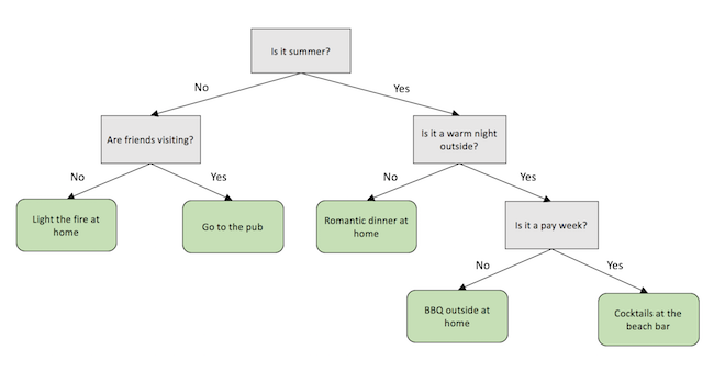
The goal of the decision tree algorithm used for classification problems (like the one we are looking at) is to create one of these decision trees to classify records into a set number of categories. To do this, it starts with all the records in the training dataset and looks through all the features until it finds the one that allows it to most ‘cleanly’ split the records according to their categories. For example, if you are using daily weather data to try and determine whether it will rain the following day (i.e. there are two categories, ‘it does rain’ and ‘it does not rain’), the algorithm will look for a feature that best splits the records (in this case representing days) into those two categories. When it finds that feature, and the value to split on, it creates one point (‘decision node’) on the decision tree. It then takes each subpopulation and does the same thing again, building up a tree until either all the records are correctly classified, or the number in each subpopulation becomes too small to split. Below is an example decision tree using the described weather data to predict if it will rain tomorrow or not (thanks to Graham Williams’ excellent Rattle package for R):
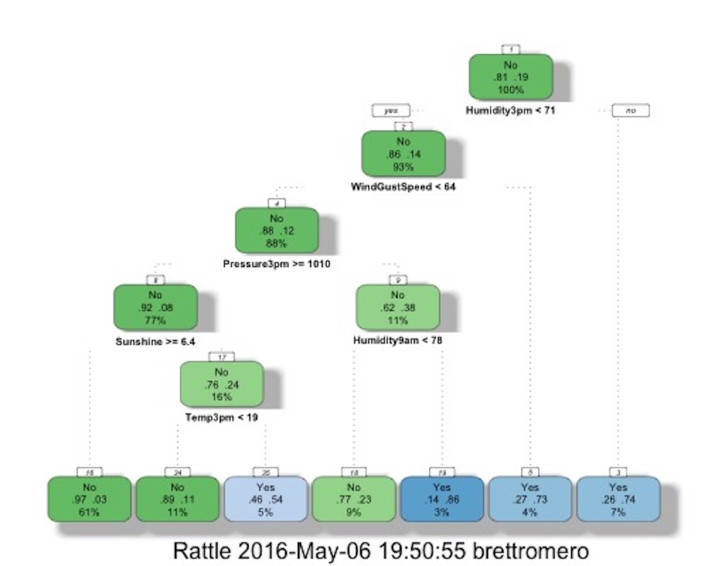
The way to interpret the above tree is to start at the top. The first criteria the algorithm splits on is the humidity at 3pm. Starting with 100% of the records, if the the humidity at 3pm is less than 71, as it is the case for 93% of the records, we move to the left and find the next decision node. If the humidity at 3pm is greater than or equal to 71, we move to the right, which takes us to a leaf node where the model predicts that there will be rain tomorrow (‘yes’). We can see from the numbers in the node that this represents 7% of all records, and that 74% of the records that reach this node are correctly classified.
The first thing to note is that the model does not accurately predict whether it will rain tomorrow for all records, and in some leaf nodes, it is only slightly better than a coin toss. This is not necessarily a bad thing. The biggest problem that data scientists have with decision trees is the classic problem of overfitting. In the example above, parameters have been set to stop model splitting once the population of records at a given node gets too small (minimum split) and when a certain number of splits have occurred (‘maximum depth’). These values have been set at values to prevent the tree from growing to large. The reason for this is that if the tree gets too large, it will start modelling random noise and hence will not work for data not in the training dataset (it will not ‘generalize’ well).
To picture what this means, imagine extending the example decision tree above further until the model starts splitting out single records using criteria like ‘Humidty3pm = 54’ and ‘Humidty3pm = 31’. That type of decision node may work for this particular training data because there is a specific record that meet that criteria, but it is highly unlikely that it represents any predictive ability and so is unlikely to be accurate if applied to other data.
All this discussion of overfitting with decision trees does however raise an important problem. That problem is how do you know how large you should grow the tree. How do you set the parameters to avoid overfitting but still have an accurate model? The truth is that is is extremely difficult to know how to set the parameters. Set them too conservatively and the model will lose too much predictive power. Set them too aggressively and the model will start overfitting the data.
Seeing the Forest for the Trees
Given the limitations of decisions trees and the risk of overfitting, it may be tempting to think “why bother?” Fortunately, methods have been found to reduce the risk of overfitting and increase predictive power of decisions trees and the two most popular methods both have the same basic premise – to train multiple trees.
One of the most well known algorithms that utilizes decision trees is the ‘random forest’ algorithm. As the name suggests, the algorithm constructs a large number of different trees (as defined by the user) by randomly selecting the features that can be used to build each tree (as opposed to using all the features for each tree). Typically, the trees in a random forest also have the parameters set to ensure each tree will also be relatively shallow, meaning that the algorithm creates a large number of shallow decision trees (decision bonsai?). Once the trees are constructed, each tree is used to predict the outcome for a new record, with these multiple predictions then serving as votes, with a majority rules approach applied.
Another algorithm which has become almost the default algorithm of choice for Kagglers, and is the type of the model we will use, uses a method called ‘boosting’, which means it builds trees iteratively such that each tree ‘learns’ from earlier trees. To do this the algorithm builds a first tree – again typically a shallower tree than if you were going to use a one tree approach – and makes predictions using that tree. Then the algorithm finds the records that are misclassified by that tree, and assigns a higher weight of importance to those records than the records that were correctly classified. The algorithm then builds a new tree with these new weightings. This whole process is repeated as many times as specified by the user. Once the specified number of trees have been built, all the trees built during this process are used to classify the records, with a majority rules approach used to determine the final prediction.
It should be noted that this methodology (‘boosting’) can actually be applied to many classification algorithms, but has really grown popular with the decision tree based implementation. It should also be noted there are different implementations of this algorithm even just using trees. In this case, we will be using the very popular XGBoost algorithm.
Alternative Models
So far we have only covered decision trees and decision tree-based algorithms. However, there are a range of different algorithms that can be used for classification problems. Given this is supposed to be a short blog series, I will not go into too much detail on each algorithm here. But if you want more information on these algorithms, or other algorithms that I haven’t covered here, there is a growing amount of information online. I also strongly recommend the Data Science specialization offered by John Hopkins University, for free, on Coursera.
K-Nearest Neighbors
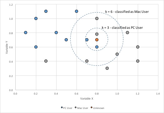
The K-nearest neighbor algorithms are arguably one of the simplest algorithms in concept. The algorithm classifies a given object by looking at the classification of the k most similar records[1] and seeing how those records are classified. This type of algorithm is called a lazy learner because during the training phase, it essentially just stores the data provided. Only when a new object needs to be classified does the algorithm start looking through the data to try to find the closest matches.
Neural Networks
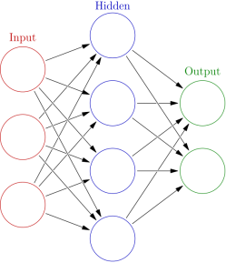
As the name suggests, these algorithms simulate biological networks by creating a series of nodes and connecting them together. A neural network typically consists of three layers; an input layer, a hidden layer (although there can be multiple hidden layers) and an output layer.
A model is trained by passing records through the network and weights adjusted at each node continually adjusted to ensure that the record ends up at the right ‘output node’.
Support Vector Machines
This type of algorithm, commonly used for text classification problems, is arguably the most difficult to visualize. At the simplest level, the algorithm tries to draw straight lines (or planes for classifications with more than 2 features) that best separate the classes provided. Although this sounds like a fairly simplistic approach to classifying objects, it becomes far more powerful due to the transformations (sometimes called a ‘kernel trick’) the algorithm can apply to the data before drawing these lines/planes. The mathematics behind this are far too complex to go into here, but the Wikipedia page has some nice visuals to help picture how this is working. In addition, this video provides a nice example of how a Support Vector Machine can separate classes using this kernel trick:
Creating the Model
Back to the modelling – now that we know what algorithm we are using (XGBoost algorithm for those skipping ahead), let talk about the approach.
Cross Validation
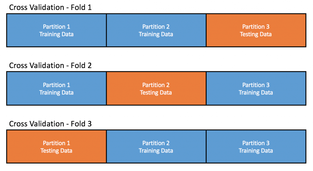
As mentioned in regards to decision trees, one of the keys risks when creating models of any type is the risk of overfitting. One of the primary ways data scientists will guard against overfitting is to estimate the accuracy of their models on data that was not used to train the model. To do this they typically use a method called cross validation. There are different methods for doing cross validation, but the method we will employ is called k-fold cross validation.
k-fold cross validation involves splitting the training data into k subsets (where k is greater than or equal to 2), training the model using k – 1 of those subsets, then running the model on the subset that was not used in the training process. Because all of the data used in the cross validation process is training data, the correct classification for each record is known and so the predicted category can be compared to the actual category. Once all folds have been completed, the average score across all folds is taken as an estimate of how the model will perform on other data. An example of a 3-fold cross validation is shown below:
Parameter Tuning
As you may have realized from the earlier description of the XGBoost algorithm – there are quite a few options (parameters) that we need to define to build the model. How many trees to build? How deep should each tree be? How much extra weight will be attached to each misclassified record? Tuning these parameters to get the best results from the model is often one of the most time consuming things that data scientists do. Fortunately, the process can be automated to a large degree so that we do not have to sit there rerunning the model repeatedly and noting down the results. Even better, using the Scikit-Learn package, we can merge the parameter tuning and cross validation steps into one, allowing us to search for the best combination of parameters while using k-fold cross validation to verify the results.
Training the Model
In order to train the model (using cross validation and parameter tuning as outlined above), we first need to define our training dataset – remembering that we previously combined the training and test data to simplify the cleaning and transforming process. To feed these into the model, we also need to split the training data into the three main components – the user IDs (we don’t want to use these for training as they are randomly generated), the features to use for training (X), and the categories we are trying to predict (y).
# Prepare training data for modelling
df_train.set_index('id', inplace=True)
df_train = pd.concat([df_train['country_destination'], df_all], axis=1, join='inner')

id_train = df_train.index.values
labels = df_train['country_destination']
le = LabelEncoder()
y = le.fit_transform(labels)
X = df_train.drop('country_destination', axis=1, inplace=False)
Now that we have our training data ready, we can use GridSearchCV to run the algorithm with a range of parameters, then select the model that has the highest cross validated score based on the chosen measure of a performance (in this case accuracy, but there are a range of metrics we could use based on our needs).
# Grid Search - Used to find best combination of parameters
XGB_model = xgb.XGBClassifier(objective='multi:softprob', subsample=0.5, colsample_bytree=0.5, seed=0)
param_grid = {'max_depth': [3, 4, 5], 'learning_rate': [0.1, 0.3], 'n_estimators': [25, 50]}
model = grid_search.GridSearchCV(estimator=XGB_model, param_grid=param_grid, scoring='accuracy', verbose=10, n_jobs=1, iid=True, refit=True, cv=3)

model.fit(X, y)
print("Best score: %0.3f" % model.best_score_)
print("Best parameters set:")
best_parameters = model.best_estimator_.get_params()
for param_name in sorted(param_grid.keys()):
    print("\t%s: %r" % (param_name, best_parameters[param_name]))
Please note that running this step can take a significant amount of time. Running the algorithm with 25 trees takes around 2.5 minutes for each cross validation on my Macbook Pro. Running the script above with all the options specified will likely take well over an hour.
Making the Predictions
Now that we have trained a model based on the best parameters, the next step is to use the model to make predictions for the records in the testing dataset. Again we need to extract the testing data out of the combined dataset we created for the cleaning and transformation steps, and again we need to separate the main components for the model. After these steps, we use the model created in the previous step to make the predictions.
# Prepare test data for prediction
df_test.set_index('id', inplace=True)
df_test = pd.merge(df_test[['date_first_booking']], df_all, how='left', left_index=True, right_index=True, sort=False)
X_test = df_test.drop('date_first_booking', axis=1, inplace=False)
X_test = X_test.fillna(-1)
id_test = df_test.index.values

# Make predictions
y_pred = model.predict_proba(X_test)
As you may have noted from the code above, we have used the predict_proba method instead of the usual predict method. This is done because of the way Kaggle will assess the results for this particular competition. Rather than just assessing one prediction for each user, Kaggle will assess up to 5 predictions for each user. In order to maximize the score, we will use the predicted probabilities that predict_proba produces to select the 5 best predictions. Finally, we will write these results to a file that will be created in the same folder as the script.
#Taking the 5 classes with highest probabilities
ids = [] #list of ids
cts = [] #list of countries
for i in range(len(id_test)):
    idx = id_test[i]
    ids += [idx] * 5
    cts += le.inverse_transform(np.argsort(y_pred[i])[::-1])[:5].tolist()

#Generate submission
print("Outputting final results...")
sub = pd.DataFrame(np.column_stack((ids, cts)), columns=['id', 'country'])
sub.to_csv('./submission.csv', index=False)
For those that wish to, you should be able to submit the file produced from this script on Kaggle. The competition is now finished and you will not receive an official position on the leaderboard, but your results will be processed and you will be told where you would have finished.
Wrapping Up
Those that are more experienced with data science may realize this series, as lengthy as it is, does not even scratch the surface of a lot of topics related to data science. Unsupervised learning, association rules mining, text analytics and deep learning are all topics that have not been covered at all. Unfortunately, the full scope of data science and machine learning are not something that can be covered in a blog. That said, I did have two goals for those reading these blog articles.
Firstly, I hope that this series demystifies some aspects of data science for those that currently see it as a black box. Although one can spend their career working in data science and still not master all aspects, even a cursory understanding of how machine learning algorithms work can help provide understanding as to what sort of questions machine learning can help to answer, and what sort of questions are problematic.
Secondly, I hope this series encourages some of you to dig deeper, to learn more about this topic. Machine learning is a rapidly growing field that is expanding to every aspect of life. This includes, recommendation engines on websites, astronomy – where it helps to identify stars and planets, the pharmaceutical industry – where it is being used to predict which molecular structures that are likely to produce useful drugs, and maybe most famously, in training self‑driving cars to drive in the real world. Whatever your primary interest, there is likely to be some machine learning applications being developed or being used already.
[1] There are a range of metrics that can be used to do this. For available metrics in the Scikit Learn package, see here.
Full script:
import pandas as pd
import numpy as np
import xgboost as xgb

from sklearn import cross_validation, decomposition, grid_search
from sklearn.preprocessing import LabelEncoder

####################################################
# Functions #
####################################################
# Remove outliers
def remove_outliers(df, column, min_val, max_val):
    col_values = df[column].values
    df[column] = np.where(np.logical_or(col_values<=min_val, col_values>=max_val), np.NaN, col_values)

    return df

# Home made One Hot Encoder
def convert_to_binary(df, column_to_convert):
    categories = list(df[column_to_convert].drop_duplicates())

    for category in categories:
        cat_name = str(category).replace(" ", "_").replace("(", "").replace(")", "").replace("/", "_").replace("-", "").lower()
        col_name = column_to_convert[:5] + '_' + cat_name[:10]
        df[col_name] = 0
        df.loc[(df[column_to_convert] == category), col_name] = 1

    return df

# Count occurrences of value in a column
def convert_to_counts(df, id_col, column_to_convert):
    id_list = df[id_col].drop_duplicates()

    df_counts = df[[id_col, column_to_convert]]
    df_counts['count'] = 1
    df_counts = df_counts.groupby(by=[id_col, column_to_convert], as_index=False, sort=False).sum()

    new_df = df_counts.pivot(index=id_col, columns=column_to_convert, values='count')
    new_df = new_df.fillna(0)

    # Rename Columns
    categories = list(df[column_to_convert].drop_duplicates())
    for category in categories:
        cat_name = str(category).replace(" ", "_").replace("(", "").replace(")", "").replace("/", "_").replace("-", "").lower()
        col_name = column_to_convert + '_' + cat_name
        new_df.rename(columns = {category:col_name}, inplace=True)

    return new_df

####################################################
# Cleaning #
####################################################
# Import data
print("Reading in data...")
tr_filepath = "./train_users_2.csv"
df_train = pd.read_csv(tr_filepath, header=0, index_col=None)
te_filepath = "./test_users.csv"
df_test = pd.read_csv(te_filepath, header=0, index_col=None)

# Combine into one dataset
df_all = pd.concat((df_train, df_test), axis=0, ignore_index=True)

# Change Dates to consistent format
print("Fixing timestamps...")
df_all['date_account_created'] = pd.to_datetime(df_all['date_account_created'], format='%Y-%m-%d')
df_all['timestamp_first_active'] = pd.to_datetime(df_all['timestamp_first_active'], format='%Y%m%d%H%M%S')
df_all['date_account_created'].fillna(df_all.timestamp_first_active, inplace=True)

# Remove date_first_booking column
df_all.drop('date_first_booking', axis=1, inplace=True)

# Fixing age column
print("Fixing age column...")
df_all = remove_outliers(df=df_all, column='age', min_val=15, max_val=90)
df_all['age'].fillna(-1, inplace=True)

# Fill first_affiliate_tracked column
print("Filling first_affiliate_tracked column...")
df_all['first_affiliate_tracked'].fillna(-1, inplace=True)

####################################################
# Data Transformation #
####################################################
# One Hot Encoding
print("One Hot Encoding categorical data...")
columns_to_convert = ['gender', 'signup_method', 'signup_flow', 'language', 'affiliate_channel', 'affiliate_provider', 'first_affiliate_tracked', 'signup_app', 'first_device_type', 'first_browser']

for column in columns_to_convert:
    df_all = convert_to_binary(df=df_all, column_to_convert=column)
    df_all.drop(column, axis=1, inplace=True)

####################################################
# Feature Extraction #
####################################################
# Add new date related fields
print("Adding new fields...")
df_all['day_account_created'] = df_all['date_account_created'].dt.weekday
df_all['month_account_created'] = df_all['date_account_created'].dt.month
df_all['quarter_account_created'] = df_all['date_account_created'].dt.quarter
df_all['year_account_created'] = df_all['date_account_created'].dt.year
df_all['hour_first_active'] = df_all['timestamp_first_active'].dt.hour
df_all['day_first_active'] = df_all['timestamp_first_active'].dt.weekday
df_all['month_first_active'] = df_all['timestamp_first_active'].dt.month
df_all['quarter_first_active'] = df_all['timestamp_first_active'].dt.quarter
df_all['year_first_active'] = df_all['timestamp_first_active'].dt.year
df_all['created_less_active'] = (df_all['date_account_created'] - df_all['timestamp_first_active']).dt.days

# Drop unnecessary columns
columns_to_drop = ['date_account_created', 'timestamp_first_active', 'date_first_booking', 'country_destination']
for column in columns_to_drop:
    if column in df_all.columns:
        df_all.drop(column, axis=1, inplace=True)

####################################################
# Add data from sessions.csv #
####################################################
# Import sessions data
s_filepath = "./sessions.csv"
sessions = pd.read_csv(s_filepath, header=0, index_col=False)

# Determine primary device
print("Determining primary device...")
sessions_device = sessions[['user_id', 'device_type', 'secs_elapsed']]
aggregated_lvl1 = sessions_device.groupby(['user_id', 'device_type'], as_index=False, sort=False).aggregate(np.sum)
idx = aggregated_lvl1.groupby(['user_id'], sort=False)['secs_elapsed'].transform(max) == aggregated_lvl1['secs_elapsed']
df_primary = aggregated_lvl1.loc[idx, ['user_id', 'device_type', 'secs_elapsed']].copy()
df_primary.rename(columns = {'device_type':'primary_device', 'secs_elapsed':'primary_secs'}, inplace=True)
df_primary = convert_to_binary(df=df_primary, column_to_convert='primary_device')
df_primary.drop('primary_device', axis=1, inplace=True)

# Determine Secondary device
print("Determining secondary device...")
remaining = aggregated_lvl1.drop(aggregated_lvl1.index[idx])
idx = remaining.groupby(['user_id'], sort=False)['secs_elapsed'].transform(max) == remaining['secs_elapsed']
df_secondary = remaining.loc[idx, ['user_id', 'device_type', 'secs_elapsed']].copy()
df_secondary.rename(columns = {'device_type':'secondary_device', 'secs_elapsed':'secondary_secs'}, inplace=True)
df_secondary = convert_to_binary(df=df_secondary, column_to_convert='secondary_device')
df_secondary.drop('secondary_device', axis=1, inplace=True)

# Aggregate and combine actions taken columns
print("Aggregating actions taken...")
session_actions = sessions[['user_id', 'action', 'action_type', 'action_detail']]
columns_to_convert = ['action', 'action_type', 'action_detail']
session_actions = session_actions.fillna('not provided')
first = True

for column in columns_to_convert:
    print("Converting " + column + " column...")
    current_data = convert_to_counts(df=session_actions, id_col='user_id', column_to_convert=column)

    # If first loop, current data becomes existing data, otherwise merge existing and current
    if first:
        first = False
        actions_data = current_data
    else:
        actions_data = pd.concat([actions_data, current_data], axis=1, join='inner')

# Merge device datasets
print("Combining results...")
df_primary.set_index('user_id', inplace=True)
df_secondary.set_index('user_id', inplace=True)
device_data = pd.concat([df_primary, df_secondary], axis=1, join="outer")

# Merge device and actions datasets
combined_results = pd.concat([device_data, actions_data], axis=1, join='outer')
df_sessions = combined_results.fillna(0)

# Merge user and session datasets
df_all.set_index('id', inplace=True)
df_all = pd.concat([df_all, df_sessions], axis=1, join='inner')

####################################################
# Building Model #
####################################################
# Prepare training data for modelling
df_train.set_index('id', inplace=True)
df_train = pd.concat([df_train['country_destination'], df_all], axis=1, join='inner')

id_train = df_train.index.values
labels = df_train['country_destination']
le = LabelEncoder()
y = le.fit_transform(labels)
X = df_train.drop('country_destination', axis=1, inplace=False)

# Training model
print("Training model...")

# Grid Search - Used to find best combination of parameters
XGB_model = xgb.XGBClassifier(objective='multi:softprob', subsample=0.5, colsample_bytree=0.5, seed=0)
param_grid = {'max_depth': [3, 4], 'learning_rate': [0.1, 0.3], 'n_estimators': [25, 50]}
model = grid_search.GridSearchCV(estimator=XGB_model, param_grid=param_grid, scoring='accuracy', verbose=10, n_jobs=1, iid=True, refit=True, cv=3)

model.fit(X, y)
print("Best score: %0.3f" % model.best_score_)
print("Best parameters set:")
best_parameters = model.best_estimator_.get_params()
for param_name in sorted(param_grid.keys()):
    print("\t%s: %r" % (param_name, best_parameters[param_name]))

####################################################
# Make predictions #
####################################################
print("Making predictions...")

# Prepare test data for prediction
df_test.set_index('id', inplace=True)
df_test = pd.merge(df_test[['date_first_booking']], df_all, how='left', left_index=True, right_index=True, sort=False)
X_test = df_test.drop('date_first_booking', axis=1, inplace=False)
X_test = X_test.fillna(-1)
id_test = df_test.index.values

# Make predictions
y_pred = model.predict_proba(X_test)

#Taking the 5 classes with highest probabilities
ids = [] #list of ids
cts = [] #list of countries
for i in range(len(id_test)):
    idx = id_test[i]
    ids += [idx] * 5
    cts += le.inverse_transform(np.argsort(y_pred[i])[::-1])[:5].tolist()

#Generate submission
print("Outputting final results...")
sub = pd.DataFrame(np.column_stack((ids, cts)), columns=['id', 'country'])
sub.to_csv('./submission.csv',index=False)
Leave a Reply