Author: Brett Romero (Page 6 of 11)

Why Australians Love Foster’s and Other Beer Related Stories

June 25, 2015 / Brett Romero / 0 Comments

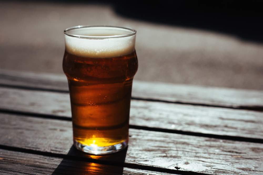
Sports. Hot summer days. Manly men. Attractive women. Whether beer is your go-to drink or not, it’s hard to not be impressed with how beer manufacturers have ensured their product is strongly associated with a range of desirable situations and topics for the average male consumer. But, despite being a common theme across countries, there are two in particular that have really taken this message to heart, to the point of being comical: Australia and the US.

Australia and the US are two countries where beer has become almost synonymous with the notion of being a “man”. Our sporting heroes appear in ads selling beer, our favorite sports teams are sponsored by beer, and when it’s not sports, it’s scantily clad women, beaches, blokes being blokes, or all three together.

But perhaps the most interesting aspect of the beer culture in these two countries is that, despite the similarities, there is an amazing mutual lack of understanding between the two. Australians for the most part have nothing but disdain for American beer – which from their perspective consists only of Bud, Miller and Coors (someone particularly familiar with international beer might venture “oh, but I don’t mind that Sierra Nevada”). Meanwhile most Americans’ knowledge of Australian beer starts and ends with a Foster’s at the Outback Steakhouse.

Both are woefully uninformed views. Hopefully, the following 1800-odd words can help clear up a few of the myths and misunderstandings – and add some mutual appreciation.

Australian Perceptions of American Beer

Mention American beer to an average Australian and you are likely to hear the words “tasteless”, “weak”, “watery” and “yellow fizzy water”, among other things not suitable for a professional blog. And let’s be honest, looking at a list of the top 10 beers in the US (see Table 1), it is hard to argue with those sentiments – the list is full of light (light carb for Australian readers) and relatively flavorless American style lagers[1].

Table 1 – Top 10 US Beers by Volume

	Label	ABV	Type	Producer
1	Bud Light	4.2%	Light Lager	Anheuser–Busch InBev
2	Coors Light	4.2%	Light Lager	Molson Coors
3	Budweiser	5.0%	American Adjunct Lager	Anheuser–Busch InBev
4	Miller Light	4.2%	Light Lager	SABMiller
5	Corona Extra	4.6%	American Adjunct Lager	Anheuser–Busch InBev
6	Natural Light	4.2%	Light Lager	Anheuser–Busch InBev
7	Busch Light	4.1%	Light Lager	Anheuser–Busch InBev
8	Michelob Ultra Light	4.2%	Light Lager	Anheuser–Busch InBev
9	Busch	4.3%	American Adjunct Lager	Anheuser–Busch InBev
10	Heineken	5.0%	Euro Pale Lager	Heineken International

Unfortunately, it is these top 10 mass produced beers that come to mind when Australians (and most people outside the US) think about American beer. That is a shame because what many Australians are completely missing out on is the absolutely massive and amazing craft beer scene that is thriving in the US.

Craft Beer in the US

Despite appearing to be a recent phenomenon, the American craft beer scene has been making its mark since the mid-90s. After declining for much of the 20^th century, the craft beer scene exploded from 446 breweries in 1993 to 1,514 by 1998. After a lull through the early and mid 2000’s, the numbers again took off in 2008 and 2009. By 2014, there were 3,464 breweries in the US.

By comparison, in Australia (depending on who you ask) there are between 100 and 200 breweries. There are at least 4 states in the US that have more breweries than the whole of Australia[2]. Craft beer also has a significantly larger proportion of the US beer market than in Australia (11% vs. 2-3%). In fact, when you look at just how big craft brewing has already become in the US (and it is still growing at a rapid pace), it makes headlines in Australian papers like “Has the craft beer machine reached saturation point?” seem a little ridiculous.

Asides from the pure numbers though, arguably the most admirable aspect of the craft brewing scene in the US is the way small breweries and brewpubs become a point of reference for the local area. In Australia, craft beer is still largely seen as the domain of inner city hipsters and beer snobs. In the US, bars and pubs will often take pride in ensuring they have the offerings from the local brewery on tap. For beer lovers, this means travelling the US provides a veritable smorgasbord of different craft beers that change with every town and season.

American Perceptions of Australian Beer

Mention Australian beer to an American, and you are likely to hear exactly one word: “Foster’s”. More knowledgeable Americans might venture that they have heard Foster’s isn’t actually that popular in Australia, which is both true and untrue. Let me explain.

Foster’s Lager, the beer most Americans (and basically everyone not from Australia) associate with Australia is a beer produced by the Foster’s Group. What many don’t know is that the Foster’s Group actually produces a large range of beers under different labels in Australia, most of which make no mention of the name “Foster’s”. Looking at the top 10 Australian beers (see Table 2), you will notice that 5 of the top 10 beers in Australia are produced by Foster’s, and in particular their largest brewery – Carlton & United Breweries[3].

Table 2 – Top 10 Australian Beers by Volume

	Label	ABV	Type	Producer
1	XXXX Gold	3.5%	American Adjunct Lager	Lion Nathan
2	VB	4.9%	American Adjunct Lager	Foster’s
3	Carlton Draught	4.6%	American Adjunct Lager	Foster’s
4	Tooheys New	4.6%	American Adjunct Lager	Lion Nathan
5	Tooheys Extra Dry	4.6%	American Adjunct Lager	Lion Nathan
6	Carlton Mid	3.5%	Light Lager	Foster’s
7	Carlton Dry	4.5%	American Adjunct Lager	Foster’s
8	Corona Extra	4.6%	American Adjunct Lager	Anheuser–Busch InBev
9	Pure Blonde	4.6%	Light Lager	Foster’s
10	Hahn Premium Light	2.6%	Light Lager	Lion Nathan

However, despite the popularity of Foster’s beer, it is actually very rare to find Foster’s Lager in Australia anymore. In fact, the only place many Australians are likely to find it is in the imported beer section of the local supermarket or bottle-o.

But this wasn’t always the case – up until the mid 80s Foster’s Lager was actually a very popular beer in Australia and was sold as a premium label amongst Foster’s other offerings. It wasn’t sold with the ubiquitous “Australian for Beer” branding, but it did have some pretty classic advertising – take a minute to relive 1980s Australia through this classic Foster’s TV spot from 1984:

So how did Foster’s Lager go from a mainstream beer to the imported section? In the mid 80s, due to changes in the Australian beer market and how Foster’s was marketing their various beers, Foster’s Lager started to lose popularity domestically as the company focused on promoting other labels such as Carlton Draught and Victoria Bitter (VB). As the then Foster’s CEO Trevor O’Hoy explains in an interview in 2006 (emphasis mine):

“Foster’s Lager had grown up as a mainstream Australian beer, punching at equal weight with VB in our portfolio. When we took it overseas, however, we took the brand slightly up-market and played heavily on ‘brand Australia’ – with international advertising featuring Paul Hogan, iconic Australian imagery and the ‘Australia’s famous beer’ tagline. That turned Foster’s into a top 10 international beer brand.

The flipside to this success was that Foster’s became the beer Australians drank overseas, not at home. Our Australian sales teams focused on the mainstream brands such as Carlton and VB, as well as innovating in cold filtered, craft brewing, dry, low carb and the light and mid categories. Foster’s Lager really didn’t have a champion or new positioning in Australia and its volumes slipped from the late 80s onwards.”

One final footnote to the Foster’s story, in December 2011, Foster’s became a subsidiary in the world’s second largest brewer by revenues, SABMiller[4]. Sadly, this means that the vast bulk of the beer being drunk by Australians is now owned by non-Australian multinationals.

Why isn’t Craft Beer Big in Australia?

As mentioned earlier, the craft beer scene in Australia is relatively small and under developed when compared to the US, even accounting for population differences. Yet Australia is a wealthy country with a healthy love for beer, so why hasn’t craft beer taken off in Australia like it has in the US?

A big part of the problem is the huge market share of the two biggest beer producers in Australia, Lion Nathan and Foster’s, and how aggressively they protect that market share.

A key weapon used by the big two to maintain market share is the tap or pourage contract, something that would be illegal in the US. When negotiating to supply beer to a bar, hotel or pub, a contract will be agreed to that sees the brewer provide rebates and other benefits[5] to the venue owner in exchange for securing exclusive access to most, if not all, of the taps. As an end consumer, this often means that Foster’s or Lion Nathan will own every beer (and cider) on tap at your regular watering hole.

A second key to maintaining market share is the willingness of Lion Nathan and Foster’s to buy out smaller brewers that are proving popular. Even many Australians will be surprised to learn that beers they thought were coming from small independent breweries (White Rabbit, Little Creatures, Bees Knees, Fat Yak, Knappstein, Matilda Bay) are in fact owned by Lion Nathan and Foster’s.

Competing against these two giants, craft breweries fighting to get access to taps, with typically more expensive small batch products, are often left with the choice of continuing to scrape out a living selling by the bottle, or selling out altogether. Even when a craft brewery does manage to get access to a tap, venue owners are often made generous offers to boot them in favor of another label from the big brewery that has locked up the other taps.

An example of how difficult it can be for craft brewers to get and maintain access to taps was provided in an excellent article by Adele Ferguson in the Sydney Morning Herald last year. The following is an excerpt from that article detailing the experience of a pub owner in Melbourne:

“Sitting down to his computer, a Melbourne publican discovered an email waiting for him. Sent by an executive from Carlton & United Breweries (CUB), it contained an offer that left him gobsmacked.

One of CUB’s specialty brews had been ”selling very well” in other pubs, the email explained. It then suggested the publican sell that brew on tap – at the expense of a specific competing craft beer that the publican was already offering. ”I’ll donate the first keg,” the CUB executive offered.”

Positive Changes Brewing?

Despite the duopoly in the Australian beer market, craft brewers are having some impact on the Australian beer market. The presence of viable craft breweries with a wider range of beers available has forced the big breweries to significantly diversify their offerings. As a result, even though all the beers on tap may be from the same company, there is typically a much wider range of offerings today then there was even 10 years ago.

And things could be about to get significantly better for craft brewers. The Australian Competition and Consumer Commission (ACCC) is rumored to be investigating whether tap contracts and other anti-competitive practices are legal under the Competition and Consumer Act. Even if they are found to be legal under the current law, the fact that these practices have been exposed is likely to create pressure for new regulations to be developed to help craft brewers survive and thrive.

For those that have seen the diversity and creativity on display in the US craft beer market, any change that gives craft brewers in Australia a better chance would be very welcome.

Classic Beer Adverts

Finally, for those looking for some light entertainment, I spent some time digging around YouTube for some classic Australian beer commercials. Unfortunately the older ads are few and far between, but I did find a top 10 from the last 10 or so years. Enjoy:

[1] Before Australian readers get too smug, they may want to sneak a look at their own top 10 (see Table 2) – it makes for equally dismal reading

[2] California – 431, Washington – 256, Colorado – 235, Oregon – 216

[3] See, the title wasn’t lying to you, Australian’s do love Foster’s

[4] Yes, that Miller

[5] Business development allowances, tickets to sporting events, promotional gear etc

US Labor Market Update – The Grind Continues

June 16, 2015 / Brett Romero / 0 Comments

On June 5, the Federal Reserve released its latest Employment Situation Summary. The results were slightly better than expected – 280,000 jobs added in the month of May compared to an expected 226,000. There were also small upward revisions to the previously released numbers for March and April.

In terms of the long-term trends in the participation rate identified previously (see here), this update didn’t really change much. The participation rate has more or less stopped falling over the past 12 months, currently sitting at just under 63% (see Chart 1). The percentage of the civilian non-institutional population[1] that is employed continues to climb slowly back towards to 60%, but is still well below the peak of over 63% reached in 2007.

Chart 1 – Participation Rate vs. Employed as Percentage of Civilian Population

The benchmark unemployment rate for May was 5.5%, a slight increase from 5.4% in April and was matched by a slight increase in the number of people unemployed, up to 8.7 million. Even though this goes against the general downwards trend in unemployment since 2010, Chart 2 shows how this slight uptick doesn’t really impact on the broader trend.

Chart 2 – Unemployment Rate

Unemployed Breakdown

Looking at the breakdown of the unemployed (see Chart 3), the average period of unemployment continuing to normalize, with the number of people unemployed for 5-14 weeks now below the number unemployed for less than 5 weeks. The group of people unemployed for 15 weeks or more, although still large by historical standards, also continues to fall in both percentage and absolute terms. To provide some indication of just how far the size of this group has fallen, in mid-2010 there were over 9 million people who had been unemployed for 15 weeks or more. That number is now less than 4 million, a decrease of over 55%.

Chart 3 – Unemployed Persons by Length of Unemployment

The improving situation for the unemployed is also evident in the average weeks people spend unemployed (see Chart 4).

Chart 4 – Average Period of Unemployment

Industry Breakdown

In Pa rt 4 of this series, we looked at what was happening to the number of people employed in various industries in the US economy. Chart 5 provides an update for some of the more interesting stories from that piece.

Chart 5 – Employment by Various Industries

By and large we see long standing trends continuing. Manufacturing continues to undergo a renaissance, bucking a long downwards trend. Nearly 1 million jobs have been added since the low point in early 2010. Education and health services, and professional and business services continue to grow strongly, while the government sector is basically still going nowhere.

Previously, we also looked in some detail at the Information sector, in particular the technology related subsectors. Chart 6 shows the breakdown of the information sector and its various subsectors.

Chart 6 – Employment in the Information Sector

What Chart 6 reveals is that the ‘Other information services’ subsector is clearly adding jobs at a fast pace, with data processing, hosting and related services also increasing employment. Chart 7 shows the employment growth rate in these two subsectors combined since 2006.

Chart 7 – Tech Subsectors Employment Growth

Since 2011, these sectors have been adding jobs at an annualized rate of between 6% and 8%. In total this has led to a 35% increase in jobs in these sectors since the start of 2011 – which is fantastic growth. But these subsectors are starting from a very low base –a 35% increase only translates into an additional 139,000 jobs. By way of comparison, over that same period, professional and business services added over 2.6 million jobs, education and health services added 1.9 million and even manufacturing added 700,000 jobs.

One thing to keep in mind though is that the tech boom is causing jobs to be created in other fields that service the technology sector. Lawyers, accountants, talent recruiters and HR personnel, among others, all provide support to the technology sector. Most of these roles are likely to sit in the professional and business services, which we just saw has added a lot of jobs. A big part of that story could be the tech boom.

[1] Persons 16 years of age and older residing in the 50 states and the District of Columbia, who are not inmates of institutions (e.g., penal and mental facilities, homes for the aged), and who are not on active duty in the Armed Forces.

Australian Housing Bubble – Further Reading

June 15, 2015 / Brett Romero / 0 Comments

Over the past 2-3 months, the mainstream media coverage of housing prices in Australia has exploded. Every commentator appears to have had a piece on this topic and was waiting for the right time to publish it. That right time is apparently now. For those interested in additional reading on this topic, here are some of the better pieces I’ve come across:

The banks and real estate: a Ponzi scheme that could ruin us? – Ian Verrender | ABC News

The housing crash we had to have: A Gen Y perspective on the bubble – Matt Ellis | Rational Radical

Another interest rate cut will fuel a housing bubble in danger of bursting – Greg Jericho | The Guardian

It’s not Hockey’s job comment that should worry us most – Michael Janda | ABC News

Blowing bubbles: the tricky task of tackling Sydney’s property market – Amy Auster | The Conversation

4 charts of the ‘largest housing bubble on record’ – Wolf Richter | Wolf Street

The Sydney housing bubble to pop – but how? – Michael Pascoe | The SMH

The mother of all housing bubbles – Chris Joye | The Australian Financial Review

Women and Corruption Issues in Kosovo

June 11, 2015 / Brett Romero / 0 Comments

For those that don’t know, over the past couple of months I have been spending time working with a tech startup/NGO here in Pristina called Open Data Kosovo. The main aim of the organization is to encourage and facilitate the release of data and other information by the government of Kosovo (and related bodies) in order to increase transparency and reduce corruption. So far they have been fantastically successful, getting both national and international media attention, which is all the more impressive when you consider they are only now coming to the end of their first year of existence.

One of the main things I have been working on since joining is putting together some analysis of the various datasets they have been publishing online to see what conclusions can be provided to the public that might help create a more informed discussion of the issues. The first piece has now been published on the Open Data Kosovo website and we are excited to see what kind of feedback we get. If you want to take a look, please click the link below:

More women in leadership would probably reduce corruption, but is there a more effective way?

Australian Housing Bubble Redux

June 9, 2015 / Brett Romero / 3 Comments

In the recent piece about the Australian economy we touched on the issue of the bubble in Australian house prices. Over the weekend, Saul Eslake, Chief Economist at Bank of America Merrill Lynch and one of Australia’s most respected economists, added his thoughts to the debate. A lot of his concern is around the longer term affects on people who are locked out of the housing market:

“I would say [rising house prices] are causing social harm because they are widening the gap between those who have houses and those who don’t, and freezing younger generations out of home ownership,”

In a country like Australia where, much like the US, owning your house is seen as a noble goal that everyone should be able to achieve, this could signal a cultural change. Home ownership in Australia is at its lowest level since 1950 as investors increasingly snap up properties, not for the rent/income they will generate, but for the assumed capital gains. In recently released data from the Australian Taxation Office (ATO) for the 2012-13 financial year, 1,967,260 (or just over 15% of all taxpayers) claimed rental income. Of those, 64% declared a net loss (i.e. they claimed deductions for negative gearing). Think about that for a second – almost 2 out of every 3 people with an investment property in Australia are actively losing money on that investment. What do these investors do if their expectation of further capital gains changes?

“2 out of every 3 people with an investment property in Australia are actively losing money on that investment.”

With all these statistics, why is there still an argument about whether a housing bubble exists? A big part of the problem is that there is no qualitative measure of a bubble. In hindsight they tend to be blindingly obvious, but one of the reasons bubbles occur at all is that most people don’t notice them as they are inflating. Adding to the problem is the reluctancy of politicians and commentators to call out bubbles or even use the word ‘bubble’ because of the negative connotations – bubbles tend to burst. The following was the response of Australian Assistant Treasurer Josh Frydenberg when asked about the possibility of a housing bubble on the ABC Insiders program on Sunday morning:

“I don’t think there is a housing bubble… In the early 2000s housing prices increased by 20 per cent for three years in a row and then were steady for a decade. And there wasn’t a bubble that led to a major correction.”

However, as the situation becomes more extreme, more and more respected commentators are starting to sound the alarm on this issue, even if they avoid calling it a bubble. Saul Eslake again:

“What I do say, without any hesitation at all, is that Australian prices of housing in most Australian cities, and particularly in Sydney, are, as [Reserve Bank governor] Glenn Stevens called them in September last year, ‘elevated’,”

So, leaving aside talk of bubbles, what are the facts?

Australians have record levels of housing debt as a percentage of income
Almost 2 out of 3 property investors are losing money on their properties
The median house price in Sydney is now over AU$900,000
Rates of home ownership are at their lowest levels in over 60 years

Whether or not you want to call it a bubble, that seems unsustainable to me.

Why the RBA doesn’t want to cut rates

June 6, 2015 / Brett Romero / 0 Comments

The first Tuesday of the month is interest rate day in Australia, the day the Reserve Bank of Australia – the Australian equivalent of the Federal Reserve – announces any changes to the official cash rate. The decision for June was to leave interest rates on hold at 2.0%.

In a situation that will feel relatively alien to readers in the US, Australian interest rates have never really been close to 0, but have been falling since late 2011 (see Chart 1).

Chart 1 – Australian Cash Rate vs. US Federal Funds Rate

What has been leading to falling rates in Australia over a period where the US has been slowly recovering and the Fed Reserve is slowly edging back to normalizing interest rate policy? As is usually the case, a mix of factors are involved.

Iron Ore and Coal Prices Return to Earth

A story that most people outside Australia have at least heard about is the large mining boom Australia has been enjoying over the past decade or so, and that it was largely driven by demand from China. What they may not know is that this mining boom has been largely driven by just two commodities (well technically three) – iron ore and coal (two types of coal – thermal and metallurgical). Chart 2 shows the prices of iron ore and thermal coal[1] in AUD/tonne since the 1995.

Chart 2 – Iron Ore and Thermal Coal Prices 1995 to Present

From this chart, we can clearly see the huge increase in prices that boosted the Australian economy. This was particularly pronounced for iron ore which went from between AU$16-AU$17 a tonne for most of the 90s to over AU$180 a tonne in 2010 and 2011.

Aside from generating huge profits for anyone who happened to own a coal or iron ore mine, what this price rise also led to was a large amount of employment in areas that weren’t just digging up the commodities themselves. This included:

Exploration of possible new mining sites – at AU$180 a tonne everyone wanted an iron ore mine
Building infrastructure that facilitated the large-scale digging up and exportation of these commodities – ports needed to be built and/or expanded, mining pits dug, roads paved and so on
Providing services to mining companies – lawyers, accounts, caterers and so on

After peaking in 2010/11 though, things started to go into reverse. By late 2013, much of the investment in infrastructure had run its course and the people who were employed to build that infrastructure were no longer needed. Prices were falling, bringing into question the viability of a lot of higher cost mines (and the mining companies running these mines) set up during the boom period. In short, a lot of people formerly employed on mine sites or in mining services roles were finding themselves looking for a new job and the rest of the economy was (and still is) struggling to pick up the slack. This in part is because of the …

High Exchange Rate

For those that haven’t decided to brave the 20+ hours of flight time to visit Australia in the recent past, Australia has become an extraordinarily expensive place. Sydney and Melbourne have been consistent fixtures in the world’s most expensive cities to live lists over the past 10 years.

Most of this was driven by a very strong Australian dollar, which was in turn driven mostly by the mining boom. In addition to buyers of commodities needing Australian dollars to buy the products they wanted, Australia became the target of a large volume of carry trade with currency traders looking for a relatively stable economy to park money at a relatively high interest rate. As a result of this, at the height of the mining boom, the AUD was buying almost $1.10USD.

Since that peak, the Australian dollar has depreciated around 30% (see Chart 3), easing a lot of the price pressure. However, as of 2015, Sydney and Melbourne still rank 5^th and 6^th on the world’s most expensive city list, as provided by the Economist Intelligence Unit’s (EIU) bi-annual Worldwide Cost of Living report.

Chart 3 – AUD/USD Exchange Rate 1995 to Present

The RBA has publically been stating that they believe the value of the Australian dollar is too high in an attempt to talk down the value of the Australian dollar (often called ‘jawboning’) and provide a boost to the non-mining sectors of the Australian economy. They have also progressively lowered the cash rate from 4.75% in 2011 to 2.0% today, in an attempt to stem the carry trade. As we have seen, to some degree they have been successful, but the exchange rate is still higher than they (and many other commentators) believe is optimal.

Unfortunately, some bumbling on the part of the RBA (or the execution of a plan that no one else understands) has blunted some of their efforts. At the previous monetary policy meeting at the start of May, the RBA lowered the official cash rate from 2.25% to 2.0%, but removed any talk of further cuts from the publically released meeting minutes (removing the “easing bias”). Doing this then had the opposite of the desired result and caused a spike in the Australian dollar.

Chart 4 – Consumer price index; year-ended change 2000 to 2015

So why are they removing the easing bias? Why don’t they just slash rates further – after all inflation is running below the target band (see Chart 4)? The problem is they are worried about the…

Bubble in House Prices

The RBAs hesitancy to cut interest rates further is mostly due to a concern about further encouraging investment in housing and contributing to rising house prices, which look to be well into bubble territory.

For those that aren’t too familiar with Australia, particularly the modern, post ‘put-another-shrimp-on-the-Barbie’, Australia, being a property tycoon has become something of a national obsession. Home renovation shows are everywhere and are getting huge ratings. Morning news regularly holds interviews with the latest property ‘success story’.

This obsession has led to Australia becoming a world-beater when it comes to levels of household debt. The Australian Bureau of Statistics (ABS) produced a great series of charts in May 2014 showing some alarming statistics. See below for some of the highlights:

Chart 5 – Household Debt vs. Annual Income[2] in Australia 1987 to 2013

Charts 6 and 7 – Household Debt vs. Annual Income – Various Countries 2001 to 2013

After 20 years of Australians continually buying properties off each other for ever-increasing prices, funded mostly by increasing level of mortgage debt, something changed. Perhaps it was the median house price in Sydney soaring past AU$900,000 (approximately US$700,000 at today’s exchange rate). What ever triggered it, in recent months, the talk in Australia has become all about a bubble in house prices, particularly in Sydney and parts of Melbourne. The Secretary of the Department of the Treasury, John Fraser, recently became the latest high profile public figure to weigh in:

“When you look at the housing price bubble evidence, it’s unequivocally the case in Sydney, unequivocal,”

More over, he drew a direct link between high house prices and low interest rates:

“It does worry me that the historically-low level of interest rates are encouraging people to perhaps over-invest in housing,”

And there is plenty of evidence to support the notion that the rise in housing prices is increasingly due to investors as opposed to owner-occupiers (see Chart 8).

Chart 8 – Investor Housing Credit as a Percentage of Total Housing Credit 1990 to 2014

Meanwhile, belying the sparkling reputation the Australian Government has earned internationally in recent times[3], the Government has all but ruled out taking any meaningful action to reverse key policies that are currently encouraging investment in property – negative gearing and the capital gains tax concession being two of the main culprits. When asked in a recent session of question time by the leader of the Opposition Bill Shorten to respond to the comments from John Fraser, Prime Minister Tony Abbott responded as follows:

“As someone who, along with the bank, owns a house in Sydney I do hope our housing prices are increasing,”

Summing Up

All this leaves the RBA in quite a pickle. Relatively high interest rates (by the standards of developed nations internationally) continue to keep the exchange rate at higher than desired levels, which makes Australia an expensive place to do business. This in turn harms Australia’s two big non-commodity exports – higher education and tourism – just when they need to pick up the slack from a cooling mining sector. But lowering interest rates risks further fueling a bubble in house prices which the Government seems quite happy to ignore.

I don’t imagine there are too many people who would like to be in the shoes of RBA Governor Glenn Stevens right now.

Keep an eye on this space for further updates as this all unwinds.

[1] This is an example of that classic Australian trait – sarcasm

[2] Gross disposable household income received during the previous year.

[3] If anyone can find a good historical price series for metallurgical coal, I’d love to hear from you

Labor Statistics Part IV – The Employed

May 25, 2015 / Brett Romero / 0 Comments

Previously in Parts II and III, we focused on two subsets of the population that are not employed – non-participants and the unemployed. In Part IV, we finally move on to looking at the population of employed people. However, in a slight change of tack, instead of focusing on the characteristics of these people, we are going to look at the changes in the employment market in general and more specifically at the changes at the industry level.

Declining Industries

Chart 1 – Industries with Declining Shares of the Employment Market 1939 to 2015

Decline in Manufacturing

Looking at the data, the big story since the end of World War II (1945 for those who skipped History class) is the decline of the manufacturing industry. Manufacturing was far and away the biggest sector in the US in terms of employment at the end of the war, but has seen its share of the employment market decline to less than 9% as of 2015. The reasons for this have been the subject of a lot of discussion (see here for example), but if we look at the number of manufacturing jobs (see Chart 2), as opposed to the percentage of the non-farm employment market, we see there are two phases to this decline.

Chart 2 – US Manufacturing Jobs 1939 to 2015

As Chart 2 makes clearer, manufacturing in the US was actually still adding jobs from 1945 through to the late 70s, it was just that the other sectors were adding more jobs, causing the manufacturing sector’s share of the employment market to decline.

From the mid 80s onwards though, the manufacturing sector started declining in both percentage and absolute terms. Increasing automation and the shift of jobs to low cost manufacturing countries such as China, India and other developing nations started what would be a long decline for the industry. There is one ray of light though, and that is that the US has actually been adding manufacturing jobs for the past 6 years. Although this looks like a positive change, it is hard to say whether this is the start of a new trend or just an aberration representing the recovery of jobs lost in the last downturn. The 90s boom saw similar gains before they were reversed very quickly in the new century.

Where is the Tech Boom?

The sector that you may be surprised to see in the declining chart is the Information sector. Information Technology (“tech”) seems to be the only sector that anyone is talking about right now – glitzy product launches, podcasts (the excellent Startup) and TV shows (Silicon Valley is fantastic if you haven’t seen it). So why don’t we see it in the employment data? To explain that, it helps to break the sector down into its component industries (see Chart 3).

Chart 3 – Information Sub Industries, All Employees 1990 to 2015

The finer level data only goes back to 1990, but this is the key period we are interested in anyway. What we see is that despite the hype, the two tech related sub industries (Data processing, hosting and related services, and Other information services) are still very small, even within the Information sector. In terms of the number of people employed, these two sectors are drowned out by the traditional publishing industry and the telecommunications sector. So even though the two tech sub industries have been adding jobs, it has simply not been enough to outweigh the job losses in the larger sub industries.

The Telecommunication Boom

The other interesting point on Chart 3 is how much the tech boom in the late 90s impacted on the telecommunications sector. Despite the popular perception that this boom was a tech boom (it is called the dot com bubble after all), the boom led to far greater increases in job numbers (and job losses after the bust) in the telecommunications sector than in the tech sectors. The boom in telecommunications was primarily driven by telecom companies rushing to upgrade networks and infrastructure in response to exploding demand for the two hot new products of the time: the internet and mobile phones. After the bubble popped, some large companies went bust, others consolidated, but the net result was a lot of job losses.

Expanding Industries

Chart 4 – Industries with Expanding Shares of the Employment Market 1939 to 2015

Moving on from declining industries, let’s look at the industries that have grown their share of the employment market over the past half a century. The clear winners here are the Education and Health sector, and the Professional and Business Services sector.

Professional and Business Services

Professional and Business Services cover a range of services that have gone from non-existent, or the domain of niche firms, to being the domain of some of the world’s largest firms. Additionally, being employed to provide services within this sector has become very prestigious (legal services and management consulting are good examples), allowing these firms to attract some of the top talent in the market place.

Overall, the growth in the number of people employed to provide these services is largely explained by the increasing complexity of doing business. Increasing complexity creates demand in several ways, including the need for:

People who are experts in one or a small subset of specific business functions
People who are experienced in navigating an increasingly complex regulatory environment, and/or
Agility to quickly respond to certain business needs that preclude hiring and training staff internally

In recent times there has been talk about larger businesses attempting to ‘in-house’ some of the services that professional services firms typically provide, particularly legal services and various compliance functions. As of yet, this does not appear to be impacting the employment growth of professional services firms.

Inexorable Rise of Education and Health

The Education and Health sector has shown the strongest and most consistent growth of any industry over the last 50 years. But what explains this strong growth? Chart 5 provides a breakdown of the subsectors within this industry.

Chart 5 – Education and Health Sub Industries, All Employees 1990 to 2015

The first thing to note is that all the sub sectors have been adding a large number of jobs over the past 25 years, but there are two standouts:

Social Assistance (child care workers, personal and home care aides, social and human service assistants) has gone from easily the smallest sub-sector in 1990 to employing as many people as the Education sub-sector, tripling the number of people employed.
Ambulatory Health Care Services (outpatient medical services like dentists, GPs, diagnostic centers and so on) has become easily the largest sub-sector over the past 25 years, adding over 4 million jobs.

Generally this provides further confirmation of what we saw in Part II of this series – that there are larger numbers of Americans retiring and as they do, the demand for certain services, particularly health care is also growing.

Childcare Catch 22

One additional point to make on this subject is regarding the growth in childcare services, a key component of the overall growth of the sector. As the model of the family has changed to one with two parents in full-time employment, there has been a corresponding growth in demand for childcare services. For a lot of families this has presented a question – is it worth paying for childcare (does the parent earning the least still earn more than the cost of childcare?).

This causes a catch 22 for the childcare industry in most countries – childcare typically struggles to attract enough suitable employees due to a combination of parents’ (understandably) high expectations and generally low pay. However, if businesses in the childcare industry were to offer higher pay to childcare workers to attract more candidates, they would need to raise the cost of the childcare to parents, leading to more parents simply dropping out of the workforce to stay home and raise their children instead. Because of a parent’s ability to provide their own childcare services, without Government intervention, it will be difficult for the wages of childcare workers to ever significantly exceed the average income for parents in the area they service.

The Financial Sector Reflects the Market

The last sector I want to spend some time on in this section is the financial sector. One of the noticeable things from Chart 4 is, as a percentage of the total non-farm employment market, the financial sector hasn’t grown since the late 80s. This would seem to contrast with the general notion of an ever-expanding financial sector that is taking over the US economy. Again, the fact that we are looking at the data in terms of the percentage of total non-farm employees can be deceptive. Chart 6 shows the total financial sector employees from 1990 to 2015.

Chart 6 – Financial Sector, All Employees 1990 to 2015

Looking at this chart, we see the Financial sector did add a significant number of jobs between 1990 and 2015, but the number of jobs in the financial sector is still relatively small compared to the economy as a whole. Additionally, the number of jobs in the Finance sector appears to change in line with with the economy as a whole. Does that mean the Financial sector doesn’t need to be reigned in or that it isn’t sucking talent out of the US economy into relatively unproductive industry? That is a topic for a separate article, but the one thing that can be said is that in terms of the number of people being employed by the Financial sector, everything looks very much like business as usual.

Stable Industries

Chart 7 – Industries with Stable Shares of the Employment Market 1939 to 2015

The Government Sector

Despite there being observations we could make about both the other two industries on this chart, I am going to focus on the most interesting story on this chart – the Government sector. The basic story in the chart is the build up in the percentage of non-farm employees in the Government sector from 1945 to the mid 70s, and then a slow decline through to 2015. Again looking at the percentages can be deceiving, so let’s look at the number of employees in the Government sector (Chart 8):

Chart 8 – Government Sector, All Employees 1955 to 2015

The period from 1955 to 2009 saw a pretty consistent build up in the Government sector – close to 15 million jobs were added in this time. But since 2009, ignoring census hiring in 2010 (you can also see corresponding spikes in all years ending with ‘0’ for the same reason), the number of people employed by the Government had its biggest decline since the early 80s. To help determine what is happening, let’s look at the Government sector broken down into its three sub-sectors, Local, State and Federal (see Chart 9):

Chart 9 – Government Sub Sectors, All Employees 1955 to 2015

At first this would seem to show a slightly confusing picture. This decline from early 2009 through to late 2014 represents almost 6 years right in the middle of Barrack Obama’s presidency, but for all the noise about political stalemate in Washington, the sequester and the Government shutdown, there appears to have been minimal impact on the number of Federal Government employees. At the same time, Local Governments have been slashing payrolls and State Governments have essentially been in a hiring freeze. The explanation for this is largely due to:

The nature of Local and State Government revenue sources – the three main types of taxes that Local and State Governments collect are income tax, forms of sales tax, and property tax. All three sources took sharp downturns in the recession, with property tax continuing to decline even as income and sales tax collections were recovering.
Balanced budget requirements – many State and Local Governments have balanced budget requirements, which meant in the face of sharply falling revenues, they were forced to slash expenditures. In many cases this meant cutting payrolls, which unfortunately only exacerbated the effects of the recession locally.

The combination of sharply falling revenues and the inability to use debt financing led to large job losses at the State and Local Government level. On the other hand, it is well known that Federal Government does not have a balanced budget requirement (much to the chagrin to some on Capitol Hill) and, in contrast to the State and Local Governments, significantly increased spending going into the recession (the American Recovery and Reinvestment Act of 2009). The merits and impact of Government financed stimulus may be debated, but the impact on employment within the Government sector is pretty obvious.

A Strange Observation

The other surprising observation from Chart 9 is that the Federal Government has employed more or less the same number of people since the late 1960s – all the growth in the Government sector has come from the Local and State Government sectors. The growth in Local Government makes sense, the population of the US has increased significantly in that period and providing Governance for that population requires more employees. We also see growth in State Government for the same reasons – but nothing at the Federal level.

Technology and other efficiency gains should allow fewer people to do the same amount of work over time, and the productivity gains between now the 1960s have been huge. Additionally, the impact of these efficiencies would be greatest at the Federal level where the scale of the work is typically bigger and there is less need to maintain a physical presence all over the country/state in the same way that Local or State Government has to. But the efficiencies wouldn’t apply everywhere:

To audit the same percentage of businesses over time, the IRS would need to continually hire additional auditors to keep up with the growing number of people and businesses
For Social Security to continue to service a growing population, the number of locations (and the staff to keep them running) would also need to expand significantly

Even allowing for a more efficient work force, it seems unlikely that the Federal Government has been able to maintain the same levels of service, regulatory effectiveness and Government advisory when the country has grown so much in population and complexity.

From here it would be easy to launch into a diatribe about an understaffed Federal Government leading to issues like the financial crisis, the failure to detect various huge frauds (Enron, Bernie Madoff), and the generally poor quality of Government services (the torturous immigration process comes to mind[1]). I could then also go on to talk about how using the points above to argue for further reductions in the Federal Government seems crazily wrong-headed. However, linking all these events to a shortage of Federal Government employees is far too simplistic. These events were caused by a range of factors and simply adding more Federal public servants would not have solved the problem on its own.

All that said, not increasing staffing levels for 50+ years does have an impact. The next time you are forced to suffer through some unnecessarily archaic (Federal) Government process, read about another fraud that the SEC and/or FinCEN failed to pick up, or lament that lobbyists are writing a significant amount of legislation that gets put before congress, keep in mind that collectively the Government agencies providing these functions are today operating with the same number of people as they were when Neil Armstrong took his first steps on the moon.

[1] Please don’t tell me that this is done intentionally to discourage applicants – there are plenty of ways to discourage applicants without wasting huge amounts of time and money.

Have any thoughts on what impact constant levels of Federal Government staffing since the 1960s might have had? Please leave them in the comments!

Why You Probably Don’t Need a Financial Advisor

May 17, 2015 / Brett Romero / 0 Comments

I recently had an interesting series of conversations with my parents around investing and the world of financial advice, which encouraged me to outlay some thoughts on the subject. First things first – I am not a financial advisor, and none of this should be taken as specific investment advice. My only aim is to highlight some common mistakes people make when it comes investing. If after reading this you feel you may not be getting the best advice, your next step should be to do your own further research and/or have a more informed conversation with your current financial advisor.

Why You Probably Don’t Need a Financial Advisor

Generally speaking, financial advisors are people who provide a service to investors, helping them build, balance, manage and adjust a portfolio of assets, taking into account the prevailing economic conditions and the expectations and needs of the client. There are a multitude of scenarios where financial advisors and asset managers provide a valuable service to their clients, unfortunately, however, as Matt Yglesias points out, this is almost never for small “retail investors”, like you or me.

If this is the case, why are financial advisors still in such demand when it comes to retail investors? I believe it comes down to four factors:

Unrealistic expectations on the part of retail investors
Fear of complexity
The belief that your financial advisor’s incentives align completely with your own, and/or
A lack of understanding of compounding.

Adjusting Expectations

Your expectations may seem pretty straightforward – you want to maximize the returns on your assets. But let’s dig a little deeper – what level of returns are you looking for? For most people, the prospect of 5-7% per annum returns seems underwhelming – that’s pretty much the average for the market right? What if I want to beat the market – half the investing world is beating the market average in a given year – surely I can be one of those guys?

Unfortunately, there is no shortage of people who will tell you they can help you do exactly that. From stock pickers in your local newspaper to highly paid active fund managers on Wall St, there is an endless line of people who want to help you discover the secret of obtaining above average returns. More often than not, it is even sold as quite a reasonable thing, an opportunity that others have overlooked for some plausible sounding reason, or something that is only available to a tiny subset of investors that you happen to a part of.

The problem is not the salesmen – salesmen are gonna sell – the problem is we keep buying into the promises of above average returns, despite our own better judgment. The reality is beating the market is extremely difficult to do, particularly over any multi-year period. Even if there are advisors and money managers that have found a way to consistently beat the market, they are running a hedge fund with billions in assets, or providing advice to people and/or companies with a lot more money than you or I. They are almost certainly not working 9 to 5 at your local branch of ABC Bank.

To start thinking like an investor, instead of a gambler, the first step is to readjust your expectations. There are no shortcuts to wealth – average market returns should be your expectation. Once that is your expectation, your view on the best way to invest your money fundamentally changes. Now the question changes from “How big is the return I can get?” to “What is the lowest cost way to match the average market returns?” That is the right question to be asking.

Fear of Complexity

Fear is a tool that has been used by professionals in most fields essentially since the beginning of people doing things for money. From lawyers to auto mechanics to management consultants, they have a vested interest in making any job they do seem more complicated than it is to ensure that a) you don’t learn how to do it yourself; and b) they can charge as much as possible for their services. People working in the financial industry are no different.

That’s not to say there aren’t extremely complicated products and concepts in the financial world, but now that we have adjusted our expectations – all we want is to match average market returns – why do we need to understand these complicated products? Do you have a large exposure to Chinese Yuan that you need to hedge? Have you been creating short positions on European junk bonds that you need to cover? You can probably stop reading this if you do.

If we accept that matching the average market return is in fact a perfectly acceptable result, then there are a range of simple, understandable options available to retail investors that are only a regular brokerage account away.

The Incentive Misalignment

Despite the platitudes, a financial advisor’s primary incentive is to maximize the amount of money they make from you as a client. There is some alignment in incentives in the sense that their fees increase as your assets grow (fees are typically structured as a percentage of total assets), but the difference to your advisor between your assets growing at 5% or 7% is minimal. The real money is in finding additional pools of assets to manage. Because of this, it is much more economical for them to spend their time finding additional clients than it is for them to spend that time trying to squeeze an extra percent or two out of your portfolio. Confused? Similar incentives apply for Real Estate agents (I’m just picking fights with everyone today) as is explained very well in the following short clip.

The above misalignment is actually one of the more innocent ways in which an advisor’s incentives can diverge from your best interests. The more disturbing divergence occurs due to the opaque world of incentives and commissions. This varies widely between countries, states and even the specific type of advisor you have, but these payments can lead an advisor to recommend products and strategies that aren’t actually the best option for you[1]. This could include recommending unnecessarily complex portfolio structures, advising you to take on too little or too much risk, or even recommending funds and/or securities that the advisor actually receives commission for selling. Most people have heard about this happening in the US, but don’t believe it doesn’t happen elsewhere – take this excerpt from the Financial Services Guide for Colonial First State, an Australian Wealth Management Group (emphasis mine):

“You may receive advice in relation to the products we offer from financial advisers who do not work for Colonial First State or may be representatives of other licensees in the Bank. These advisers may receive some benefits from us. The adviser’s remuneration is included in the fees you pay when investing in our products.”

The issue here isn’t that these products are being marketed, but there is a blurring of the lines between advisor and salesman that is particularly bad in the financial industry. Again referring to Matt Yglesias – compare buying securities recommended by your advisor to buying a car: “we understand that the car salesman works for the dealership — he’s not your car advisor.”

The key point is that the only person who really cares about your money is you and you should spend as much time researching how you invest your money as you would on any other major purchase. Fortunately, there has never been a better time for investing novices to learn some of the basic concepts of investing – CNN, ASIC, Yahoo Finance and many others have beginner’s guides to investing. For those looking for something more in depth, Coursera is a fantastic resource of free courses offered by some of the worlds leading Universities. Two excellent beginners’ finance courses are currently being offered by the University of Michigan and Yale.

So instead of spending all your time online looking up Joe Pesci trivia, watching John Stewart clips on racial inequality, or researching the best toothbrush to buy, invest some time building your financial knowledge. Start with important concepts like the risk-return tradeoff and diversification, and move onto the different types of securities. Let your curiosity take you where you want… after you watch the Joe Pesci clip of course.

Underestimating Compounding

One of the big reasons so many of the injustices in the financial markets occur is because people consistently underestimate the effects of compounding. Let’s look at a simple example – the bank provides you with an asset worth $0.01, but it doubles in value every day (i.e. it would be worth $0.02 on day two, $0.04 on day three and so on) for an entire 31-day month. How much would that asset be worth at the end of the month?

If your guess had less than 7 figures, you are way off. By the end of the month, that asset would be worth over $10 million. That is the impact of compounding. Let’s look at a more relevant example for investors. Anecdotally, you will often hear people say something along the lines of the following:

“X was a great investment – it doubled in price over the last 10 years.”

What is the average rate of return that would cause an asset to double in value in 10 years? 7.18% per annum. Consistent 7.18% returns is nothing to sneeze at, but it is a lot less impressive than the returns sought by a lot of investors. It is also lower than the long run average return of the S&P500, which is over 9% (see Chart 1).

Chart 1 – Value of $100 Invested in the S&P500 in 1928

Ok, so leaving relatively small amounts of money invested at low rates results in a lot bigger returns than you might expect. If that is the case, it shouldn’t matter if my advisor is charging me 0.15% or 1.5%, as long as I leave it accumulating for long enough, right? Unfortunately the opposite is true, when it comes to fees, compounding works against you. Those seemingly small fees that financial advisors and intermediaries charge you for their services end up having a much bigger impact than you might expect.

Just as compounding works by exponentially increasing a value by giving us returns on our returns, the money lost through fees grows exponentially by taking away money each year that would be compounded in future years. Chart 2 shows a comparison of two $100,000 investments over 30 years assuming the long run returns of the S&P500 (9%). One investment is made in a low cost market index fund (cost 0.1% of assets) and the other in a high cost managed fund (cost 1.5% of assets).

Chart 2 – $100,000 Investment: High Cost vs. Low Cost Management

Within 5 years, the high cost fund has cost you over $10,000 more in fees and lost returns than the low cost fund – that’s over 10% of the value of your initial investment gone. The cost reaches over $30,000 by the 10-year mark, and over $135,000 by year 20.

The worst part of this, going back to the first point, is there is almost no chance that your high cost fund managed to outperform the market index fund over the course of those 20 years, and a pretty good shot it did significantly worse. At best you probably just paid $135,000 to match the average market returns… on the plus side, maybe they will take you out on their new yacht for your generosity.

What To Do?

If you understand and agree with the points made above, and if you are currently investing or are planning to invest any significant money, then what you should be looking for is something that will allow you to reproduce the market average performance at a very low cost. There is a growing number of ways to do this, but low cost managed funds and ETFs are the most accessible to most investors.

However, do not simply substitute this advice for your old financial advice. Do your own research – there is so much information out there, and the best advice is often free. Understand what the product options are, what the fees and costs are, and what returns are expected and why. Don’t be afraid to ask questions – the only dumb question is the one asked after you have lost a stack of money.

[1] The option recommended might simply be less beneficial than the best option as opposed to an option that is not in your interest at all, which would be a breach of fiduciary obligations.

Disagree with any of the above? Feel free to leave a comment below.

4 Economics Concepts to Improve Decision Making

May 14, 2015 / Brett Romero / 0 Comments

Rightly or wrongly, the reputation of the economics profession has taken a battering over the last 6 years. Largely this is because of the perceived inability of economists to foresee the Global Financial Crisis, and the anemic recovery that occurred afterwards in most countries. Leaving the debates over austerity vs. stimulus, liquidity traps and the zero lower bound for another day, I thought I would go back to some basic economic concepts and how, with a little bit of imagination, they can be useful in situations most people encounter in everyday life.

1. Opportunity Costs

Opportunity cost is a concept used in economics to help determine the cost of a particular action or choice. At the most basic level, the opportunity cost of doing something is the cost of NOT doing the most (economically) beneficial alternative.

For example, it is Saturday morning and you are going to drive to your friend’s house for a morning session of Call of Duty. The cost of doing this might appear to simply be the cost of gas to get there and any marginal wear and tear on the car. However, economically the cost is more than that – it also includes the benefit of the most productive activity forgone. Depending on your circumstances, that might have been picking up the breakfast shift at the local café, or putting time into that startup idea you have been working on. Whatever the case may be, you have unconsciously placed a higher value on time spent playing games then the alternative and, in many cases, that is a tangible value (the café example).

This may change nothing in your mind, you may really get a lot out of hanging out and playing games – video games are a huge industry precisely because people place a high value on playing games. But once you start consciously thinking about the cost of your actions in this manner, it tends to have an impact on how and where you spend your time.

2. Incentives

One of the parts of general economic theory that tends to rub people up the wrong way is the idea that everything can be quantified and compared. This is not a particularly romantic way to look at the world, but this line of thinking can be used to help understand and change behaviors.

For example, many people have trouble finding the motivation to go to the gym. Why is it so hard to go consistently? When you hit that sleep button on the alarm, you are making a choice based on the incentives in front of you – and you are valuing an additional hours’ sleep higher than the benefit of a gym session. There can be a range of very rational reasons for that – the benefits of any given gym session are tiny and hard to identify even if the long term benefits of consistent gym work (e.g. improved fitness, a more appealing physique) are highly valued. When you look at it that way, every morning you are faced with a choice between an immeasurably small improvement in health/fitness, or an additional hour of sleep and relaxation.

However, once we realize what the problem is, we can use incentives to reweight the choice to get the desired result. In the gym example, this can be done in a range of ways that will probably sound familiar. You can set a goal like running a half marathon – that provides additional incentive in the form of not letting yourself and/or others down or avoiding embarrassment. It could be a more immediate incentive such as treating yourself to a better lunch if you go to the gym. Organizing a gym or exercise partner will provide incentive in the form of not wanting to let your partner down by cancelling (this only really works if they don’t happen to sleep in the same bed as you). Sometimes, all that is needed is to clearly identify what the benefits will be and remind yourself of them.

Expanding this way of thinking, it can be used to look at a lot of different aspects of your life. If you have a goal to cook at home more regularly, what steps can you take to make that more appealing after a day at work (or make eating out less appealing)? Trying to commit to further study? Perhaps clearly identifying and reminding yourself of how the it will get you closer to that dream job will help provide the needed motivation.

The next logical step for this way of thinking is using it to understand the behaviors of those around you, and then utilizing that understanding to make changes. If you are a manager, how can you rearrange the incentives for the people you are managing to improve productivity or eliminate some unwanted behavior? If you have children, what incentives can you use to motivate them to help with the housework or clean up their room?

One thing to be aware of is that the incentives people are responding to can be complicated and counterintuitive. Understanding your own motivations, never mind the motivations of those around you, is something that takes time. However, the simple act of stopping to consider what may be causing you or someone else to make a choice can often lead to meaningful insights.

3. Sunk Costs

The standard definition of a sunk cost is a cost that has already been paid and is unrecoverable. In economics the concept is usually used in relation to firms (businesses), but we all deal with sunken costs on a pretty regular basis.

The classic example is where you have bought a ticket to a concert but when the day arrives you have come down with a cold (or worse). You spent all that money on the ticket so you should definitely go, right? Actually, to make the economically optimal decision in this situation, you should ignore how much you spent on the ticket (the sunk cost) and simply base your decision to go or not on whether you would still enjoy the concert more than the next best alternative (lying in bed and binge watching season 4 of the Walking Dead). Depending on how bad you are feeling, that decision could go either way.

That sounds simple right? Let’s try a thought experiment to see how difficult this can be in practice. Using the same example from above, let’s first imagine the concert ticket only cost you $10. You probably don’t have to be feeling very sick before The Walking Dead is sounding pretty appealing. Now imagine the ticket cost you $1,000. In your mind, what would it take to stop you going to that concert? Broken leg? Getting stung by an Irukandji jellyfish? If you were being rational (at least in an economic sense), you would be just as willing to forgo the concert regardless of what the ticket cost.

Applying this thinking can be tough in practice (I would have to be close to death to pass up a $1,000 concert ticket), but being conscious of it can help to avoid some poor decision-making. Should you keep pouring time and money into an unsuccessful business because you spent a bunch of money and time getting it started? You probably shouldn’t. Is it acceptable not to drink yourself into a coma after you spent money on an all-you-can-drink pass? Yes, it certainly is. It can even apply to relationships – should you continue dating your current jerk boyfriend because you have already spent 5 years with him? This isn’t a relationship advice blog, so I’ll leave that one to you, but you can see where this is going.

4. Expected Cost/Benefit

Calculating the expected cost or benefit of a set of choices can be a great way to analyze a situation where there are multiple possible outcomes, even if you don’t have specific numbers to attach to certain outcomes. Used in the right situations, it helps to identify, clarify and compare the expected outcomes of different courses of action.

Let’s look at an example where you need to decide whether to apply for a promotion or not. Let’s imagine you are in a work place and a position opens up at the next level that will be filled internally. Here is the scenario:

The next level pays $10,000 p.a. more than your current job
You are one of two people that can go for the position, but the other candidate is much better qualified and you believe they will get the job if they apply
When you speak to the other candidate, they are on the fence as to whether they want the promotion (let’s say there is a 50% chance they will apply)
Your current boss is a bit of a possessive jerk and if you apply for the job and don’t get it, you estimate he will cut your bonus by $5,000
Your current boss can also be a generous possessive jerk, and if you don’t apply, you estimate he will bump up your bonus by $2,000 for showing loyalty

Should you go for the position? We can calculate the expected benefit/cost of each course of action to help us make the decision. Here are all the possible outcomes:

	Candidate 2 Applies	Candidate 2 Doesn’t Apply
You Apply	-$5,000	+$10,000
You Don’t Apply	+$2,000	+$2,000

Given these outcomes, we can now weight the outcomes by the probability of them occurring to determine what the best course of action is:

Expected Benefit of Applying: 50% × -$5,000 + 50% × $10,000 = $2,500

Expected Benefit of Not Applying: 50% × $2,000 + 50% × $2,000 = $2,000

Based on this calculation, you should apply for the job, as the expected benefit is $500 higher than not applying.

Of course this is a stylized example, in reality it is unlikely that you have all the information given above. However, even missing some pieces of information, you can still use this approach to provide a baseline for your thinking. You may not know what the chances of the other person applying are, but by doing this calculation, you can determine that if there is anything more than a 50% chance of them applying, you will be better off not applying. You may not be able to estimate the impact on your bonus of an unsuccessful application, but you can work out how big the cut would have to be to stop you applying (a $6,000 cut in the above case) and then decide whether that is likely to occur. In short, you can use the information you do have to help you make your decision.

Initially it may be difficult to picture many scenarios where this type of thinking may be useful. However, with a little imagination, you may be surprised how often these situations present themselves. Some example scenarios may include:

Trying to buy a car knowing someone else is also interested – should I increase my offer, stick to my original low-ball offer, or pull out altogether?
Salary negotiations at work – should I accept the first offer or hold out for more money?
Deciding who to have lunch with when you are double booked – who would be the most offended and/or who can I most easily make it up to?

BONUS POINT: Getting Over Decisions That Don’t Pan Out

One of the key benefits of approaching your decision-making in a more rational, fact-based manner (aside from hopefully better decision-making) is that there will be less regret when you make a decision that does turn out badly.

Sometimes, even when you make the correct decision based on the information you have on hand, things will turn out badly – and the reverse can also be true. What changes when you start approaching your decision-making in a more calculated way is you provide yourself with an audit trail of assumptions and reasoning used. Now, instead of wondering why you made a particular decision, you can analyze the assumptions and reasoning used and work out what, if anything, went wrong. Did I underestimate how annoyed my current boss would be with me for applying for other jobs? Did I let sunk costs influence my decision? From that point, the only thing left to do is to learn and readjust for next time.

Used any other economic concepts in your day to day life? Had any interesting experiences using the ones mentioned above? Please leave a comment and share the story!

Labor Statistics Part III – The Unemployed

April 28, 2015 / Brett Romero / 0 Comments

Following on from Part II where I looked at the population of people who had left the labor force completely, this week I turn my attention to the unemployed. The unemployed are defined as those who are currently not employed but have made “specific efforts to find employment some time during the previous 4 week-period ending with the reference week”. Chart 1 maps the unemployment rate since 1948.

Chart 1 – US Unemployment Rate 1948 to 2015

Courtesy of the Bureau of Labor Statistics, there are several ways we can divide up the population of unemployed people to better understand what is driving the changes over time.

Cause of Unemployment

The first breakdown (shown in Chart 2) is the unemployed population (as a percentage of the total civilian labor force) broken down according to the cause of unemployment:

Lost a job
Left a job
Rejoining the labor force after some hiatus
Joining the labor force for the first time

Chart 2 – Unemployed Persons by Cause 1967 to 2015

From this breakdown, the first conclusion we can draw is that people losing their jobs drives almost all the variation in the total unemployment rate over time. This stands in stark contrast to the population of job leavers and new entrants to the labor force, both of which have remained remarkably consistent over a long period of time.

The second thing to note is that the changes for those reentering the labor force appear to track the changes for job losers, but with smaller peaks and troughs. This suggests that when there is a spike in people losing their jobs (due to a recession for example), a population of people who had left the labor force is returning to look for jobs. Although counterintuitive (why would you rejoin the labor force in the middle of a downturn?), this likely reflects cases such as a family where the primary breadwinner loses their job, and both parents begin the hunt for jobs to make ends meet.

This is interesting primarily because it shows a feedback loop that potentially increases the spike in unemployment in a downturn. That is, just as large numbers of people are getting laid off from their jobs, an additional population of people who weren’t in the labor force also begins looking for jobs, further boosting the population of unemployed. Conversely, this also means that unemployment can fall much quicker than anticipated (for example when one parent becomes employed and the other drops out of the labor force again).

Education Level of the Unemployed

Chart 3 shows the unemployed population broken down by education level and the obvious conclusion to draw is that your teachers were right; finishing school will help you get (and keep) a job. The rates of unemployment for those people that didn’t finish high school are significantly higher than for everyone else, keeping in mind this is for people actively looking for work (as opposed to cruising on their parents couch or living off a wealthy spouse). Conversely, the unemployment rate for those that completed a bachelor’s degree or higher is by far the lowest of the four groups.

Chart 3 – Unemployed Persons by Education Level 1992 to 2015

The other observation to be made is that there is not a huge difference in the unemployment rates for those that finished high school but didn’t go on to further studies, and those that went on to get an associates degree or attend, but not finish, college (university for those not in the US). Contrast this with the large gap between the ‘Some College/Associates Degree’ group and the ‘Bachelor’s or Higher’ group, and the advantage of graduating from college (at least in regards to getting employed) becomes plain to see.

Length of Unemployment

One of the more interesting and discussed breakdowns of the BLS unemployment data is the breakdown by length of time unemployed. Chart 3 shows how these percentages have changed over time for three groups:

Chart 4 – Unemployed Persons by Length of Unemployment 1948 to 2015

The main feature that immediately stands out on this chart is the huge spike in the percentage of people unemployed for more than 15 weeks in 2009. This peak is well well above anything since the end of World War II and remains high today. This indicates that in addition to unemployment spiking in the global financial crisis (as we saw in Chart 1), people tended to stay out of work for significantly longer than in any other downturn since the end of World War II.

What this chart also shows us is how far the US economy is from what would be considered ‘historically normal’. For most of the past 60 years, the majority of unemployed people were unemployed for less than 5 weeks, followed by those unemployed for 5-14 weeks, and then finally the smallest group was those unemployed for 15 weeks or more. However, with the financial crisis we saw this split reverse and, unlike previous downturns, over 6 years after the financial crisis the population of people unemployed for 15+ weeks is still significantly higher than the population of people unemployed for less than 5 weeks.

Further confirming this shift, an additional series that the BLS produces is the average weeks unemployed (see Chart 5). From this chart we see that the latest downturn caused a huge spike in the average weeks unemployed, but also that the average period of unemployment remains at a level higher than at any other point pre-crisis.

Chart 5 – Average Period of Unemployment 1948 to 2015

The other interesting point from Chart 5 is that even before the spike in 2009, if we look past the ups and downs of the recessions and recoveries, there appears to a trend of slowly increasing average time unemployed in the preceding 60 years. What would cause this average to creep up over time? It is likely to be a combination of a number of factors. Below are some factors that have occurred over time that could help explain this trend:

Professionalization of recruiting – recruiting is increasingly a function that is handled by a professional team within an organization, or is outsourced to a professional firm, even for smaller companies. This practice generally ensures a certain minimum standard of hire, but also means it is increasingly rare that a firm will take a chance on someone with a long period of unemployment or a spotty employment history.
Increasingly technical nature of jobs – with many professional jobs, even outside of the tech world, there is increasing pressure to continually develop new skills and adapt to new software and best practices just to keep up with the requirements of the job. As difficult as this can be for someone in the job, it is essentially impossible for someone who is unemployed leaving that person heavily disadvantaged in the job market.
Improved ability to validate work history – previously, if a person had been unemployed for an extended period, they could fudge the dates (or flat out lie) with little chance of being found out. In 2015, with online networks such as LinkedIn and generally more thorough background check processes in place, it is much more difficult to get away with this type of deception (although it definitely still happens).

Many of these changes would appear to be positive changes, such as increasing professionalism in the recruitment process and less room to mislead potential employers, so surely we are just reducing the number of dishonest people and under qualified children of bosses/friends getting jobs? That is probably true to some extent. But what is also true is that those underdog stories that we love to hear about and watch, like a mother becoming hugely successful after years of staying home to raise the kids, or a super smart kid scamming his way into a prestigious law firm, are becoming close to impossible in reality. For better or worse, the job market is becoming a place for the Louis Litts of the world, not the Mike Rosses.

People in Part Time Work

Finally, although officially classified as employed, the BLS also tracks the number of people who want full time work but that are currently only working part time (also referred to as ‘under employed’). The change in this population is shown in Chart 6.

Chart 6 – Persons at Work Part Time for Economic Reasons 1956 to 2015

One of the criticisms of the recovery post-2009 has been that it is a “part-time recovery” (see here and here for example). In other words, the belief is that the jobs being created are mostly part-time jobs and so the unemployment rate is not accurately reflecting the poor state of the economy. However, we can see that although the peak in 2009 was high (but not the highest, the peak in this series was actually 6.2% in October 1982), it has since fallen back to around average for the period and continues to fall in both absolute and percentage terms.

Watch this space for the final part of this series, Part IV, where we will explore the employed population.

Australian Perceptions of American Beer

Table 1 – Top 10 US Beers by Volume

Craft Beer in the US

American Perceptions of Australian Beer

Table 2 – Top 10 Australian Beers by Volume

Why isn’t Craft Beer Big in Australia?

Positive Changes Brewing?

Classic Beer Adverts

Chart 1 – Participation Rate vs. Employed as Percentage of Civilian Population

Chart 2 – Unemployment Rate

Unemployed Breakdown

Chart 3 – Unemployed Persons by Length of Unemployment

Chart 4 – Average Period of Unemployment

Industry Breakdown

Chart 5 – Employment by Various Industries

Chart 6 – Employment in the Information Sector

Chart 7 – Tech Subsectors Employment Growth

Chart 1 – Australian Cash Rate vs. US Federal Funds Rate

Iron Ore and Coal Prices Return to Earth

Chart 2 – Iron Ore and Thermal Coal Prices 1995 to Present

High Exchange Rate

Chart 3 – AUD/USD Exchange Rate 1995 to Present

Chart 4 – Consumer price index; year-ended change 2000 to 2015

Bubble in House Prices

Chart 5 – Household Debt vs. Annual Income[2] in Australia 1987 to 2013

Charts 6 and 7 – Household Debt vs. Annual Income – Various Countries 2001 to 2013

Chart 8 – Investor Housing Credit as a Percentage of Total Housing Credit 1990 to 2014

Summing Up

Declining Industries

Chart 1 – Industries with Declining Shares of the Employment Market 1939 to 2015

Decline in Manufacturing

Chart 2 – US Manufacturing Jobs 1939 to 2015

Where is the Tech Boom?

Chart 3 – Information Sub Industries, All Employees 1990 to 2015

The Telecommunication Boom

Expanding Industries

Chart 4 – Industries with Expanding Shares of the Employment Market 1939 to 2015

Professional and Business Services

Inexorable Rise of Education and Health

Chart 5 – Education and Health Sub Industries, All Employees 1990 to 2015

Childcare Catch 22

The Financial Sector Reflects the Market

Chart 6 – Financial Sector, All Employees 1990 to 2015

Stable Industries

Chart 7 – Industries with Stable Shares of the Employment Market 1939 to 2015

The Government Sector

Chart 8 – Government Sector, All Employees 1955 to 2015

Chart 9 – Government Sub Sectors, All Employees 1955 to 2015

A Strange Observation

Why You Probably Don’t Need a Financial Advisor

Adjusting Expectations

Fear of Complexity

The Incentive Misalignment

Underestimating Compounding

Chart 1 – Value of $100 Invested in the S&P500 in 1928

Chart 2 – $100,000 Investment: High Cost vs. Low Cost Management

What To Do?

1. Opportunity Costs

2. Incentives

3. Sunk Costs

4. Expected Cost/Benefit

BONUS POINT: Getting Over Decisions That Don’t Pan Out

Chart 1 – US Unemployment Rate 1948 to 2015

Cause of Unemployment

Chart 2 – Unemployed Persons by Cause 1967 to 2015

Education Level of the Unemployed

Chart 3 – Unemployed Persons by Education Level 1992 to 2015

Length of Unemployment

Chart 4 – Unemployed Persons by Length of Unemployment 1948 to 2015

Chart 5 – Average Period of Unemployment 1948 to 2015

People in Part Time Work

Chart 6 – Persons at Work Part Time for Economic Reasons 1956 to 2015

Archives

Categories

Tags